


A loss function, also called a cost function or error function, is a mathematical expression that assigns a numerical value representing the cost or penalty associated with a particular event, decision, or prediction. In optimization, the goal is typically to minimize the loss function to achieve the most accurate or efficient outcome. The objective function—its counterpart—may instead represent a quantity to be maximized, such as profit, accuracy, or utility.
Loss functions are central to statistics, machine learning, decision theory, and economics, where they quantify the deviation between predicted and actual values. In control theory and risk management, they define penalties for deviations from targets or undesirable outcomes.
Historical Background
The concept of the loss function dates back to Pierre-Simon Laplace, but it was formalized in statistical decision theory by Abraham Wald in the mid-20th century. Wald’s framework linked decisions, uncertainty, and loss into a unified mathematical model.
In economics, loss functions are used to model regret or cost, while in actuarial science, they estimate the difference between premiums and payouts. Since the work of Harald Cramér in the 1920s, loss modeling has become a core principle in insurance mathematics.
Common Types of Loss Functions
Quadratic Loss Function
The quadratic loss function, also known as squared error loss (SEL), measures the squared difference between a target value and a prediction:
λ(x) = C(t − x)²
where C is a constant and t is the target. This loss penalizes large errors more heavily, making it widely used in regression analysis, control theory, and statistical estimation.
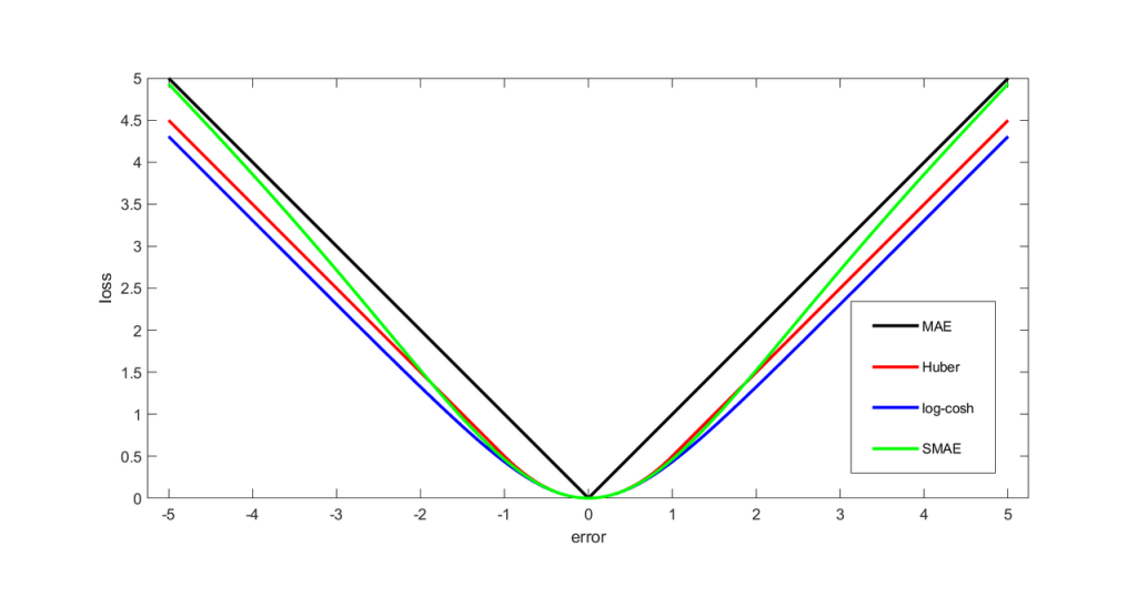
The quadratic form’s symmetry means that errors above and below the target contribute equally to the total loss. However, its sensitivity to outliers has led to the adoption of Huber, log-cosh, and smooth mean absolute error (SMAE) alternatives in modern data analysis.
0–1 Loss Function
In classification problems, the 0–1 loss function penalizes incorrect predictions with a value of 1 and correct ones with 0:
L(ŷ, y) = [ŷ ≠ y]
This loss is simple but non-differentiable, making it less practical for gradient-based optimization despite its theoretical importance in decision theory.
Constructing Loss and Objective Functions
In some contexts, loss functions are predefined by problem constraints, while in others, they must be constructed from decision-maker preferences. Economists like Ragnar Frisch and Andranik Tangian developed techniques for eliciting preference-based functions from data. Tangian’s models helped distribute university budgets and regional subsidies by optimizing fairness and efficiency using additive and quadratic objective functions.
Loss functions can incorporate utility theory, risk preferences, or multi-level hierarchies depending on application needs, ensuring the chosen function accurately represents real-world costs or deviations.
Expected Loss and Risk
In probabilistic models, the loss function often depends on random variables. Its expected value defines the risk function, guiding optimal decisions.
Frequentist Expected Loss
In the frequentist framework, expected loss (risk) is calculated as:
R(θ, δ) = Eθ[L(θ, δ(X))] = ∫ L(θ, δ(x)) dPθ(x)
where θ is a fixed parameter, δ(X) is a decision rule, and Pθ(x) represents the probability distribution of observed data. This expectation measures the average loss across repeated samples.
Bayesian Risk
Under Bayesian decision theory, expected loss integrates over the posterior distribution of parameters:
ρ(π*, a) = ∫∫ L(θ, a(x)) dP(x | θ) dπ*(θ)
The optimal decision rule minimizes this Bayesian expected loss, resulting in the Bayes Rule, which represents the best decision given both prior beliefs and observed data.
Examples in Statistics and Machine Learning
For an estimator θ̂ of a parameter θ, a quadratic loss yields a mean squared error (MSE) risk:
R(θ, θ̂) = E[(θ − θ̂)²].
Minimizing this loss produces estimators equivalent to the posterior mean in Bayesian inference.
In density estimation, the loss function often measures the L2 norm between true and estimated distributions:
L(f, f̂) = ‖f − f̂‖²₂.
This leads to the mean integrated squared error (MISE), which quantifies overall prediction accuracy across a distribution.
Decision Rules and Optimization Criteria
A decision rule selects an action minimizing expected loss based on one of several optimality criteria:
- Minimax criterion: minimizes the maximum possible loss (worst-case scenario).
- Invariance principle: ensures decisions remain consistent under transformations.
- Bayesian criterion: minimizes the expected loss under a probability-weighted parameter space.
These rules form the mathematical foundation for robust optimization, game theory, and machine learning models that aim to generalize across uncertainty.
Selecting a Loss Function
Choosing an appropriate loss function is a crucial modeling decision. The choice depends on the context, distribution of errors, and the cost of misestimation.
- Under squared error loss, the mean is the optimal estimator.
- Under absolute loss, the median becomes optimal.
- In risk-averse economics, the loss is often expressed as the negative of a utility function, emphasizing subjective preferences.
Real-world systems often exhibit non-symmetric or discontinuous losses. For instance, being late for a flight incurs a higher penalty than being early, and overdosing on a drug carries more severe consequences than underdosing. Scholars such as W. Edwards Deming and Nassim Nicholas Taleb argue that empirical realism should guide loss selection, as many natural systems display thresholds or sudden nonlinear responses rather than smooth, differentiable changes.
Mathematical Properties
For optimization algorithms, differentiability and continuity of the loss function are desirable because they allow gradient-based optimization. Common continuous forms include:
- Squared Loss: L(a) = a²
- Absolute Loss: L(a) = |a|
Each has trade-offs — the squared loss exaggerates outliers, while the absolute loss may lack smoothness at zero. Consequently, hybrid or robust loss functions (like Huber or log-cosh) are often used to balance sensitivity and stability.
Applications
Loss functions underpin nearly all areas of modern optimization and machine learning, including:
- Regression models — quantifying prediction error.
- Classification algorithms — guiding model accuracy through categorical penalties.
- Control systems — measuring deviation from desired outputs.
- Finance and risk management — modeling expected losses and portfolio optimization.
- Reinforcement learning — defining reward inverses for training agents.
By systematically linking mathematical theory to decision outcomes, the loss function remains one of the most powerful conceptual tools in predictive modeling, guiding how systems learn, adapt, and optimize under uncertainty.


